Sequence To Sequence Learning with Neural Networks

(Original Paper Published by Google in 2014)

[written by Ilya Sutskever, Oriol Vinyals, Quoc V. Le]

Hello Readers!!! Welcome back to 8^th Blog of Interpretable Blog Series.
Today we are going to discuss about sequence-to-sequence learning with neural networks in detail but in very narrative and simple way.
So, let's start!!!
As usual, lets first understand what is meant by neural networks.

Okay. So, you all are having a good idea about machine learning models. Machine learning model is nothing a but a mathematical equation whose original form of equation is close to our data (in ml terms we call it a good fit) isn’t it?

So, machine learning is about choosing correct mathematical equation which we often call machine learning model, suitable for our goal and nature of the data.
But there are some complex conditions which machine learning models / equations cannot solve. For example, recognizing objects from images having complex blend of variety of objects.
So, to solve such problems, there arrived a concept of deep learning. So deep learning is sub-branch of machine learning which uses neural networks to solve problems.
AND
Neural network is a type of computer program designed to think a little bit like human brain. Its made of different layers of tiny units called “Neurons”, and they work together to solve problems.

Here Is the very basic architecture for neural networks

A] Input Layer – Which takes input. i.e. Input X1, Input X2 and Input X3
B] Hidden Layer – This is the brain of neural network. According to each problem statement, this hidden layer can be different as this hidden layer contains blend of weighted connections which can be different for each problem.
C] Output Layer – Which provides output generated from hidden layer. i.e. Output Y1 and Output Y2

So now the question arises….

What is sequence to sequence learning?
In field of AI, sequence to sequence learning means when we are giving input of one sentence and at output, we are again getting some sentence (whether transformed OR translated). Translating languages, summarizing text, or generating responses in a conversation are some common examples of sequence-to-sequence learning.
So, readers. I believe that the idea of research paper is clear now.

Abstract:

Deep Neural Networks (DNNs) showed very good accuracy on variety of complex tasks. But they failed to give appropriate results on sequence-to-sequence mappings.
In this research paper, method is using LSTM to map input sequence (sentence) with vector of fixed dimensionality and then the last step is to decode the target sequence from the vector.
LSTM also learned sensible phrase and sentence representations that are sensitive to word order and are relatively invariant to the active and passive voice.
It is observed that when order of sentence is reversed the mappings between input sentence and output sentence are improved.

So, readers, after looking at above information, maybe you are not familiar with some of the words. So, I will explain them in one sentence.

LSTM – Long Short-Term Memory – it is a neural network specially used for sequence-based tasks.
BLEU Score (Bilingual Evaluation Understudy) – It is an evaluation metrics which gives us magnitude of similarity between human translation and machine generated translation.

Its range is [0,1]. Closer to 1 means more accurate and vice-versa.

Introduction:

Deep Neural Networks are very powerful and can easily solve problems like speech recognition, visual object detection. Main strength of DNNs is ability to perform arbitrary parallel computation of longer steps.
Despite of strength and power of DNN, they can be applied to problems whose inputs and outputs can be sensibly encoded with vectors of fixed dimensionality.
But many of the real-world problems in sequence-to-sequence learning are not having fixed dimensionality. So here there is a limitation of DNNs. Likewise, Question-Answering can also be seen as sequence to sequence learning as vector of question is mapped to vector version of answer. So therefore it was clear that domain independent method which learns sequence to sequence learning will be more helpful.
In the original paper, a straightforward application of the Long Short-Term Memory (LSTM) architecture is applied. It is showed that it can solve general sequence to sequence problems. The idea is to use one LSTM to read the input sequence, one timestep at a time, to obtain large fixed dimensional vector representation, and then to use another LSTM to extract the output sequence from that vector. The second LSTM is essentially a recurrent neural network language model except that it is conditioned on the input sequence.
The LSTM’s ability to successfully learn on data with long range temporal dependencies makes it a natural choice for this application due to the considerable time lag between the inputs and their corresponding outputs

Below is the Architecture.
Model is reading ABC as input sentence and producing WXYZ as output sentence.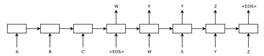

Surprisingly, the LSTM did not suffer on very long sentences, despite the recent experience of other researchers with related architectures. Researchers from the research paper were able to do well on long sentences because they reversed the order of words in the source sentence but not the target sentences in the training and test set. By doing so, they introduced many short-term dependencies that made the optimization problem much simpler.

A useful property of the LSTM is that it learns to map an input sentence of variable length into a fixed-dimensional vector representation.

Model:

RNN is a natural generalization of feedforward neural networks to sequences. Given a sequence of inputs (X1, X2, X3….Xn) a standard RNN computes a sequence of outputs (Y1, Y2, Y3…Yn) by iterating the following equation.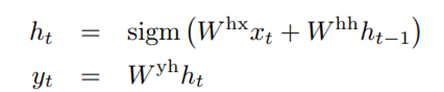

• h(t) ​ → hidden state at time step ttt (RNN’s “memory” at this step).
• sigm → sigmoid activation function (squashes values between 0 and 1). 
• W^hx → weight matrix for the input x(t)​ at time t 
• W^hh → Weight matrix for previous hidden step h(t-1)
• x(t)​ → current input.
• h(t−1) → hidden state from the previous time step.

AND
That Y(t) is our output at time t. So, readers I believe you are clear till this slide. LSTM Involves calculation of conditional probability. So before moving forward, lets understand concept of conditional probability with the help of simple one liner definition.
So, it is written as P(A|B).
What does it mean?
P(A|B) is nothing but a probability of event A if Event B has already happened.
So, coming on LSTM,

It calculates P ((Y1, Y2, Y3…Yn) | (X1, X2, X3...Xn))

So simply it means, what is probability of Y1, Y2, Y3...Yn (Predicted Output Sequence) if Input sequence (X1, X2, X3...Xn) are provided.
So, Readers. I believe that you are familiar with the basic architecture of model.

Experiments:

In research paper, they have applied method to WMT’14 English to French MT Task in two ways.

WMT’14 English to French MT refers to a machine translation benchmark task from the 2014 Workshop on Statistical Machine Translation (SMT).

One of the ways is without using SMT and One is with Using SMT (Statistical Machine Translation) and finally the results are shown.

Details Of Dataset:

For training, WMT’14 English to French Dataset is Used. Dataset of consisting of 12M Sentences consisting of 348 M French Words and 304 English Words.

Decoding And Rescoring:  

So, in original research paper things are explained with mathematical explanations. So, I decided to make it easy for you I will try to explain it in layman terms.

Once trained, they generated translations using beam search:
Beam search is a smart guessing strategy for generating sequences without checking every single possibility.
So, below are the steps. Let's see how it works.

1. Start with the beginning of a sentence.
2. Keep track of a small number B of “best guesses so far” (partial translations).
3. At each step, try adding every possible next word to each guess.
4. Throw away all but the B best guesses (based on model’s score).
5. Stop when you hit the special <EOS> (end of sentence) token.

Beam size (B) matters:

• B = 1 → simplest search (just pick the single best next word each time). Surprisingly worked well here.
• B = 2 → gave most of the improvement without much extra work.
• Larger B (B >2) → more thorough search, but more computation.
  
  

 Rescoring SMT outputs: 

They also tested another use case:

• The old SMT system produced a list of its top 1000 translations for a sentence.
• Their LSTM re-scored each translation, combining:
  
  • The old SMT score
  •  The new LSTM score (by taking an even average)

This way, their LSTM could help improve SMT results without replacing it entirely.

 Reversing the source sentences:

While LSTM is capable of solving problems with long term dependencies, it is observed that when the input sentences are reversed by keeping the target sentence as it is BLEU Score (being a performance metric for translation models) is increased from 25.9 to 30.6.
Normally, when we concatenate a source sentence with a target sentence, each word in the source sentence is far from its corresponding word in the target sentence. As a result, the problem has a large “minimal time lag”.
By reversing the words in the source sentence, the average distance between corresponding words in the source and target language is unchanged. However, the first few words in the source language are now very close to the first few words in the target language, so the problem’s minimal time lag is greatly reduced.
So here arrives new word minimal time lag. What is that?
It’s the smallest gap in time steps between when the model receives information and when it is expected to use that information to make a correct prediction.

Training Details:

They trained a large, deep LSTM model for machine translation and found it wasn’t too hard to train. The model was of 4 layers, had a lot of memory cells in each layer, and used big word embeddings. They also compared deep vs shallow LSTMs and saw big performance improvements with more layers.

Model architecture

• 4 LSTM layers (over-lapped on top of each other meaning the output of one layer becomes the input of the next).
• 1000 cells per layer — each cell is like a “memory unit” that stores information about the sequence.
• 1000-dimensional word embeddings — each word is represented as a vector with 1000 numbers, capturing its meaning.
• Vocabulary sizes:

• Input (English) vocabulary: 160,000 unique words. 
• Output (French) vocabulary: 80,000 unique words.

This means the model uses 8000 numbers to represent a whole sentence — the hidden state representation.

What’s the reason for deep LSTMs working better?

• Shallow LSTM = fewer layers.
• Deep LSTM = more layers → more processing power and more capacity to learn complex patterns.
• Every extra layer reduced perplexity by ~10% (this made significant difference)
  This is likely because of the much larger hidden state in deeper models.

Role Of SoftMax layer

• At each step, they needed to choose the next word from 80,000 possible words in the output vocabulary.
• They used a naive softmax — meaning they just computed probabilities for all words directly (no special optimization like sampled softmax).

Model size

• Total parameters: 384 million

Out of 384 million Parameters, 64 million are recurrent connections (i.e. which carry memory from previous layers)

1. 32M for the encoder LSTM - Reads the source sentence.
2. 32M for the decoder LSTM – Which are generating the translation.

Parallelization:

This module is one of the strengths of DNNs.
Let's first understand what problems they faced for implementing this parallelization.
They wrote their LSTM translation system in C++ and ran it on a single GPU. With the model from the previous section, it could process about 1,700 words / second. This speed was too slow for their needs training would take too long for getting completed.
The solution for above problem is using multiple GPUs. They had access to a machine with 8 GPUs.

They split the work across these GPUs in two main ways:

1. Layer-wise parallelization

• Their LSTM has 4 layers.
• They put one layer on each GPU.
• As soon as one GPU finished computing its layer’s output (activations), it sent the result immediately to the next GPU/layer, so no waiting for the entire batch before moving on.
  
  

2. SoftMax parallelization

• They used the other 4 GPUs to speed up the SoftMax layer (the part where the model picks the next word from the vocabulary).
• The SoftMax involved multiplying by a 1000 × 20,000 matrix (huge operation).
• They split this across the 4 GPUs so each one handled part of the vocabulary.
  
  

The result they got from that:

• Speed increased from 1,700 words/sec → 6,300 words/sec (English + French combined).
• Minibatch size: 128 sentences at a time.
• Training time: about 10 days to finish.

Experimental Results:

How they measured translation quality

• They used the BLEU score again (Billingual Evaluation Understudy)

(a standard metric for translation quality that compares model output to human translations, case-sensitive).

• They computed BLEU using the multi-bleu.pl script on tokenized text (breaking sentences into words/punctuation).
• This method is the same as in earlier important papers, and it matches the 33.3 BLEU score from when they tested that system.

Comparisons

• They tested the best WMT’14 translation system using their method of evaluation and got a BLEU score of 37.0, which is higher than the 35.8 reported on the official WMT’14 website.
• This difference is just due to slightly different evaluation scripts — not because the system actually improved.

Table 1: The performance of the LSTM on WMT’14 English to French test set (Without Use SMT (Statistical Machine Translation))

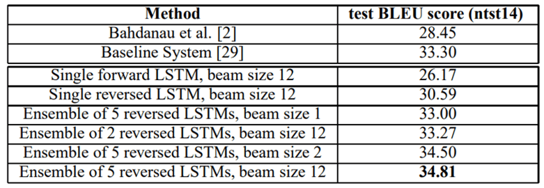
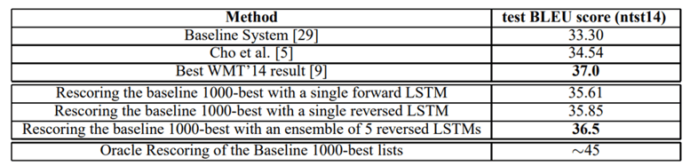
Table 2: The performance of the LSTM on WMT’14 English to French test set (With Use Of SMT (Statistical Machine Translation))

Model Analysis – Final chapter:

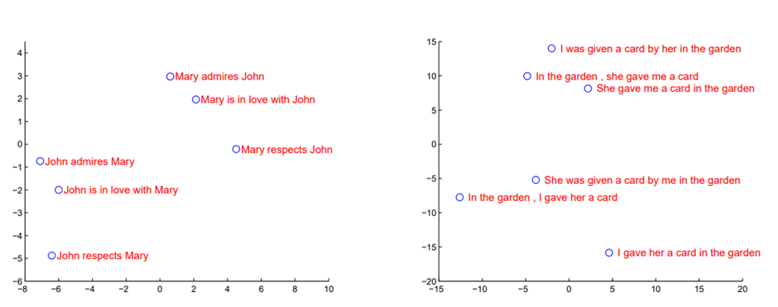
Okay Readers.

Now let's see at the model analysis graphically.

These graphs show how the LSTM groups sentences with similar meanings close together in its learned “semantic space,” even if the word order changes. Paraphrases cluster tightly, while sentences with different roles or meanings are far apart proving the model captures true sentence level meaning, not just word patterns.

Conclusion:

Large Deep LSTM’s having limited vocabulary performed well on sequence to sequence learning than SMT (Statistical Machine Translations) which are having unlimited vocabulary. It is observed that LSTMs are even doing better for longer sentences.